Jacob Gildenblat
SagivTech Ltd.
In this post we will discuss some options we have for deep learning object detection, and create a real world traffic light detector using deep learning!

One of the most important but difficult tasks in Computer Vision is object detection (also known as localization).
Object detection is about deciding where exactly in the image are objects belonging to certain categories such as cars, dogs etc.
Object detection has a long history of research and different techniques behind it.
Before the deep learning age, the object detection hype was all about cascades of haar feature detectors and then Histogram of Oriented Gradients detectors and many variants based on those.
The main idea behind these methods was using features manually designed by a human computer vision expert, and they were quite fast! Unfortunately, they were limited by the type of objects they could detect (usually rigid objects), and the number of different categories. These days deep learning is winning in this task, so let’s see if we can use it for traffic lights detection!
The deep learning object detection software eco system
Assuming we don’t want to write all that training code from scratch, we stick to existing software.
Let’s take a look at some of our options.
Single shot detectors
A very promising family of object detectors, are deep learning networks that receive an image as an input, run the network on the image, and output a list of detections.
Since these networks run through the image only once, they are referred to as “single shot” detectors.
Some notable works on this are:
- YOLO (You Look Only Once)
http://pjreddie.com/darknet/yolo/
http://arxiv.org/pdf/1506.02640.pdf - SSD (Single Shot Multibox detector)
http://github.com/weiliu89/caffe/tree/ssd
http://arxiv.org/abs/1512.02325
These object detectors were trained on the 20 categories in the Pascal VOC dataset, however you can fine tune them on your own data by changing the number of categories in the last layer of the network, possibly removing / adding layers, and retraining on your data.
To train YOLO you can use the author’s implementation in a C based deep learning framework called darknet, or one of the many ports to other packages like these:
http://github.com/xingwangsfu/caffe-yolo
http://github.com/sunshineatnoon/Darknet.keras
http://github.com/gliese581gg/YOLO_tensorflow
To train SSD it seems that only the caffe implementation is currently available online.
These detectors seem to be the most practical in terms of the runtime / quality trade-off.
However, they suffer from a common issue with deep learning algorithms – they need a lot of data.
Even if you fine tune them using the existing pre-trained networks, expect needing at least 1,000 images for each new category (if not much more) to get good results.
Sliding window approaches
Creating a sliding window heatmap from an existing classifier


This is a simple naive approach that can still be useful many times.
The scenario here is that you trained your own classifier, but want to reuse it for object detection without too much fuss.
Typical deep learning image classifiers have fully connected layers at the end of the network.
One common trick is to convert a deep learning network to be fully convolutional, by converting the fully connected layers to be equivalent convolutional layers.
The converted network can now receive larger images, and slide the original classifier across the image. The result is a score for every sliding window center location.
For more details check the Converting FC layers to CONV layers section here.
The example images above were taken from a keras implementation of this that you can use.
Now you can threshold the resulting images to get locations of your objects.
If you want invariance to scale, you can then resize the images to various sizes (larger images for detecting smaller objects) and apply the detector.
Typically you can base off an existing imagenet classifier, create a custom classifier by fine tuning it on your own data, and then use some image processing heuristics to get the most probable locations of objects in the image.
To get more accuracy, you might often need to add a new category to the classifier, which represents the background – a “not an object” category.
And now we enter an interesting zone of how to sample patches from the background.
Many windows in the image might contain only a small part of a ground truth object,
And some of them might contain two or more fractions of objects.
Our ideal detector should learn to distinguish many edge cases like these.
In the learning phase, many detectors like SSD, YOLO and even HOG, would sample random patches from the background, and use them as a “not an object” category.
Then if there are false detections, sometimes “hard negative mining” is applied, and problematic patches are given special attention.
Ideally we would want to use all the windows in the image, since that contains much more information than using just a small random subset of the windows.
To do that, we would need a clever window scoring function, that can, for example, learn that although a window contains many details from an object, there probably is a different nearby window responsible for the main part of the object.
Usually after a sliding window detection, a Non Maximal Suppression is applied, usually using a greedy algorithm.
An example of such a greedy algorithm would be to sort the windows by their scores, and keep the best scoring windows that do not overlap.
However such a greedy algorithm is not optimal (see the figure on the right).
We would want the classifier to learn an optimal Non Maximal Suppression.
A figure from the MMOD paper (see picture on the right) showing a difference between an optimal detector and a detector using greedy non maximal suppression.

Dlib’s Max Margin Object detector
Dlib is a C++ library with many computer vision and machine learning algorithms implementations.
The author of dlib, Davis King, published an algorithm called Max Margin Object Detection for solving the window scoring problem.
He then took the MMOD idea and implemented it for deep learning.
In the training phase the detector gets each of the windows in the image (as opposed to only a small random subset of windows), and each window gets scored with an appropriate objective function that aims at balancing false detections and miss detections.
This detector is able to learn nice object detectors from an absurdly low number of examples (dlib contains an example that learns a face detector from 3 images), perhaps because in the training stage the detector is fed much more windows than other deep learning algorithms.
http://blog.dlib.net/2016/10/easily-create-high-quality-object.html

Learning from only a few images? OK, let’s see if we can use dlib for traffic lights detection
Data collection
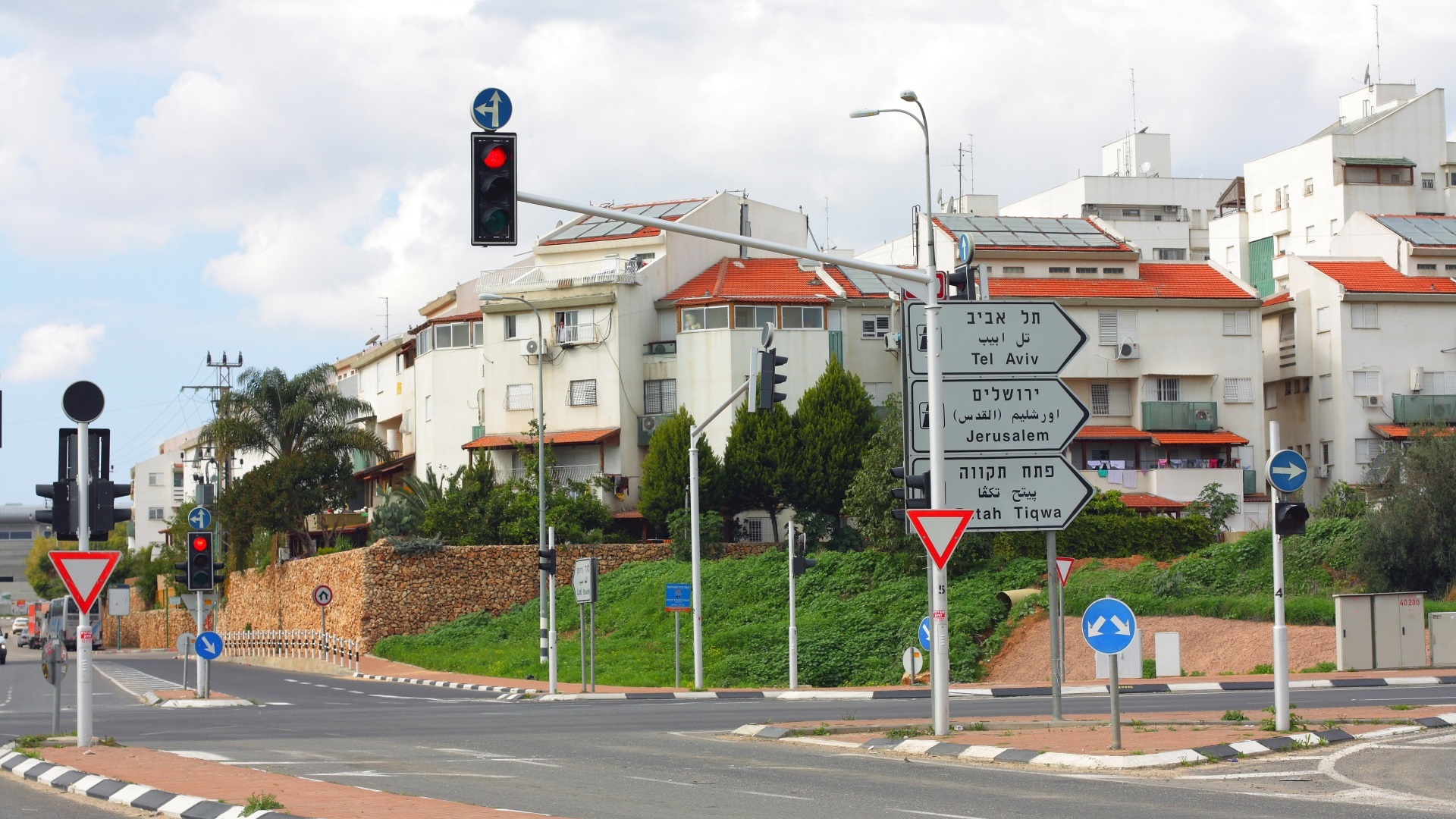
Here we take a virtual drive in google street view in some Israeli streets, and collect 30 images of traffic lights (basically just screen capturing the browser. For only 30 images, we don’t really need fancy stuff like using the street view API).
The images look like as in the picture on the left.
To mark location of the ground truth traffic lights, we used the utility provided in dlib: http://github.com/davisking/dlib/tree/master/tools/imglab
Training
Here we can use the dlib MMOD example in the dlib examples folder.
http://github.com/davisking/dlib/blob/master/examples/dnn_mmod_ex.cpp
We use a similar configuration, but changed the bounding box aspect ratio configuration to take into account that the traffic light height is much larger than its width.
We trained on 30 1600×900 images (although training on lower resolution images should be better since we will resize them in run time).
Using a Titan X, training took 3 hours.
Post processing
In testing time we resize the images to 500×300.
There seems to be an impressive ability to find traffic lights in the new images.
However there was a false positive problem, where rectangular blobs with dark frames were sometimes falsely detected as traffic lights!
To mitigate this, we applied a simple heuristic for filtering the traffic lights – the traffic lights horizontal position should be close to the center of the image.
Also, slightly blurring the image with a 3×3 Gaussian filter made the results much more stable.
Once the traffic light was detected, its state (green / red / yellow) was determined using image processing approaches – thresholding over the saturation channel (of HSV), contour finding, and peaking at the color of the contours.
Since there are many edge cases when there is overexposure or underexposure, and defining the color borders can get complex, it makes sense that the deep learning network should also learn to output the light color.
Results
Overall it seems that the detector was able to learn to detect traffic lights using an absurdly low number of 30 images!
It does seem that 30 images are too few, especially taking into account the many different combinations of poses, scales, and lights that real world examples can have.
Also the false positive problem implies that maybe the 30 images were not enough to learn the actual interior of the traffic lights (the actual light blobs!). Using one of the many deep learning visualization techniques can spill some light on that.

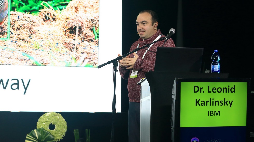
Jacob Gildenblat received his BSc. and MSc. in Electrical Engineering focusing on Computer Vision from the Tel Aviv University.
In SagivTech Jacob focuses in Computer Vision, Machine learning and GPU Computing.
Legal Disclaimer:
You understand that when using the Site you may be exposed to content from a variety of sources, and that SagivTech is not responsible for the accuracy, usefulness, safety or intellectual property rights of, or relating to, such content and that such content does not express SagivTech’s opinion or endorsement of any subject matter and should not be relied upon as such. SagivTech and its affiliates accept no responsibility for any consequences whatsoever arising from use of such content. You acknowledge that any use of the content is at your own risk.


Leave A Comment